HOMEWORK 03
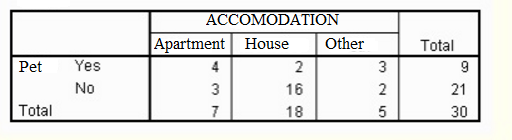
Lets start with an example! The following contingency table shows the likelihood a person in a certain type of accommodation owns a pet.
What is the conditional frequency for owning a pet, given that the person lives in a house?
We must take the number of people who owns a pet AND live in a house, then divide that number by the total number of people who live in houses: 2/18.
What’s the marginal frequency of people who live in an apartment?
Divide the number of people living an apartment by the grand total: 7/30.
What’s the number of people who has a pet and live in a House?
This is a joint frequency: it represents how many times a combination of two conditions happens together. The answe is 2.
Lets now skip to the definitions
Conditional Frequency
In a contingency table (sometimes called a two way frequency table), conditional frequency is a fraction that tells you how many members of a group have a particular characteristic. More technically, it is the ratio of a frequency in the center of the table to the frequency’s row total or column total1. To be clearer, a conditional distribution is a univariate distribution, composed by its frequency, built on the costraint of a value. It refers to a subset of the whole population.
Joint Frequency
In a bivariate distribution, given the variables X and Y, the joint frequency represents the number of statistical units which have X_i value and Y_j value at the same time. To simplify: A joint frequency is how many times a combination of two conditions happens together. For example a dog owner who is also a woman2.
Marginal Frequency
It is the ratio between the frequency of a row total or column total to the total frequency of the data. It is commonly used to analyze general trends in one specific category of data3. To simplify: A marginal frequency can be calculated by dividing a row total or a column total by the total frequency of the data4.
Statistical Indipendence
To discuss about the concept of independence between two variables (X, Y) we must refer to bivariate distributions. In a contingency table, we look at the univariate conditional distribution: significant changes among conditional distributions with a changing variable’s value means strong correlation. To simplify: if the conditional distributions has different graphs we can say that the two variables X and Y are dependant. However, if the shape of the graph are similar (or equal), we can say that there are no correlation between the variables. If this happens, conditional distributions are equal to each other, and also to the marginal one.
We can transpose this definition to frequencies. Formally: given two variable X and Y, they are indipendent if for each i, Freq(X_i, Y_j) are equal for every j. So they are also equal to the marginal Freq(X_i). Numerically:
| N(i,j)/N(+,j) == N(i,+)/N | N(i,j)/N(i,+) == N(+,j)/N |
|---|---|
These two formulas lead to
| N(i,j) x N == N(i,+) x N(+,j) |
|---|
Multipling and dividing the last formula by N, we obtain the following identity:
| Freq(X_i AND Y_j) == Freq(X_i) x Freq(Y_j) |
|---|
This is true if one X is independent from Y and vice versa. We can notice that in this case, Joint Frequencies are the product of the Marginal Frequencies.
The last formula, if transposed to probability terms, is a formal definition.
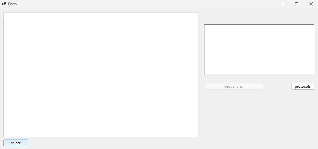
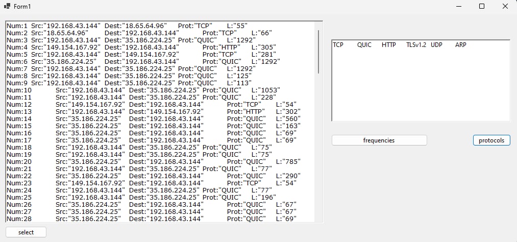
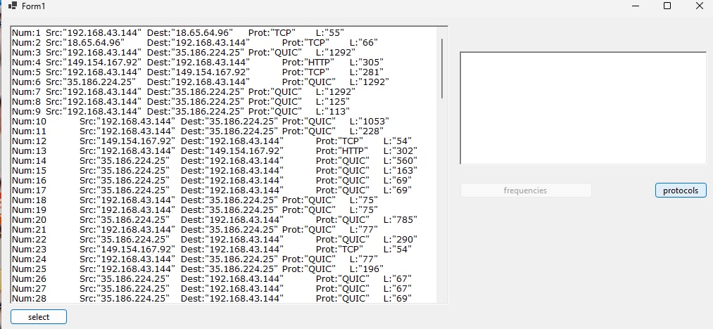
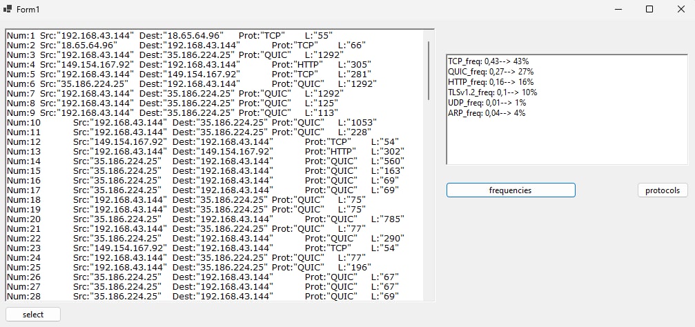
APPLICATION
A univariate distribution of protocols used among wifi’s traffic
Files are also avaible on github
Online Algorithm
An online algorithm is one that can process its input piece by piece, without having the whole dataset avaible from the start. Is it a very usefull feature as it optimize resources’ usage. In contrast, an offline algorithm is given the whole problem data from the beginning and is required to output an answer which solves the problem at hand. Insertion Sort is an example of online algorithm.
Median
In statistics and probability theory, the median is the value separating the higher half from the lower half of a data sample, a population, or a probability distribution. For a data set, it may be thought of as “the middle” value. The basic feature of the median in describing data compared to the mean (often simply described as the “average”) is that it is not skewed by a small proportion of extremely large or small values, and therefore provides a better representation of a “typical” value5.
If we can sort the data as it appears, using Insertion Sort, we can easily locate the median element. Insertion Sort is one such online algorithm that sorts the data appeared so far. At any instance of sorting, say after sorting i-th element, the first i elements of the array are sorted. The insertion sort doesn’t depend on future data to sort data input till that point. In other words, insertion sort considers data sorted so far while inserting the next element. This is the key part of insertion sort that makes it an online algorithm6.
Variance
In probability theory and statistics, variance is the expectation of the squared deviation of a random variable from its population mean or sample mean. Variance is a measure of dispersion, meaning it is a measure of how far a set of numbers is spread out from their average value, it has a central role in statistics7.
Given a sample x1,…,xN, the standard deviation is defined as the square root of the variance: 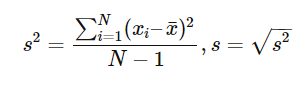
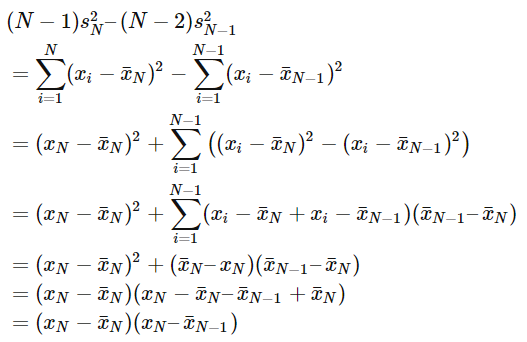
Welford’s method8 is a usable single-pass method for computing the variance. It can be derived by looking at the differences between the sums of squared differences for N and N-1 samples:
Here is provided a pseudo code for the algorithm:
variance(samples):
  M := 0
  S := 0
  for k from 1 to N:
    x := samples[k]
    oldM := M
    M := M + (x-M)/k
    S := S + (x-M)*(x-oldM)
  return S/(N-1)
and a Python implementation9:
# For a new value newValue, compute the new count, new mean, the new M2.
# mean accumulates the mean of the entire dataset
# M2 aggregates the squared distance from the mean
# count aggregates the number of samples seen so far
def update(existingAggregate, newValue):
    (count, mean, M2) = existingAggregate
    count += 1
    delta = newValue - mean
    mean += delta / count
    delta2 = newValue - mean
    M2 += delta * delta2
    return (count, mean, M2)

# Retrieve the mean, variance and sample variance from an aggregate
def finalize(existingAggregate):
    (count, mean, M2) = existingAggregate
    if count < 2:
        return float("nan")
    else:
        (mean, variance, sampleVariance) = (mean, M2 / count, M2 / (count - 1))
        return (mean, variance, sampleVariance)
Mean
For a data set, the arithmetic mean, also known as “arithmetic average”, is a measure of central tendency of a finite set of numbers: specifically, the sum of the values divided by the number of values10.
Knuth’s algorithm:
This algorithm computes the mean iteratively. This means that at each step, the value for the mean computed with the first n-1 inputs it’s updated when the input xn is received. The formula used in this algorithm is the following11: 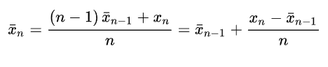
This algorithm could have a loss in accuracy because of the division operation inside the loop, but provides a smart way to calculate the mean without having the whole dataset in local storage. A pseudo code is provided:
def online_mean(data):
    n = 0
    mean = M2 = 0.0

    for x in data:
        n += 1
        delta = x - mean
        mean += delta/n
        delta2 = x - mean
        M2 += delta*delta2

    if n < 2:
        return float('nan')
    else:
        return M2 / (n - 1)
-
Statistics How To: Conditional Relative Frequency: https://www.statisticshowto.com/conditional-relative-frequency/ ↩
-
Statistics How To , Joint Frequency, https://www.statisticshowto.com/joint-frequency/#:~:text=What%20is%20Joint%20Frequency%3F,of%20two%20conditions%20happens%20together. ↩
-
Study: https://study.com/learn/lesson/conditional-joint-marginal-relative-frequency-overview-comparison-examples.html ↩
-
onlinemath4all: how to calculate marginal relative frequency: https://www.onlinemath4all.com/how-to-calculate-marginal-relative-frequency.html ↩
-
Wikipedia, Median: https://en.wikipedia.org/wiki/Median ↩
-
Geeksforgeeks: Median in a stream of integers: https://www.geeksforgeeks.org/median-of-stream-of-integers-running-integers/ ↩
-
Wikipedia, Variance: https://en.wikipedia.org/wiki/Variance ↩
-
https://jonisalonen.com/2013/deriving-welfords-method-for-computing-variance/ ↩
-
Algorithms for calculating variance: https://en.wikipedia.org/wiki/Algorithms_for_calculating_variance ↩
-
Wikipedia, Mean: https://en.wikipedia.org/wiki/Mean ↩
-
Donald Knuth, “The Art Of Computer Programming”, (1998) ↩