HOMEWORK 07

What is the Lebesgue Integral?

The Lebesgue integral plays an important role in probability theory, real analysis, and many other fields in mathematics. It is named after Henri Lebesgue (1875–1941), who introduced the integral in 1904. The usual definition of the Lebesgue integral has little to do with probability or random variables (though the notions of measure theory and the integral can then be applied to the setting of probability, where under suitable interpretations it will turn out that the Lebesgue Integral of a certain functions corresponds to the expectation of a random variable)¹. Here is an intuitive idea of what the Lebesgue integral is, as compared to the Riemann integral. Recall from Calculus the idea behind the Riemann integral: the integral $\int_a^b f(x) \, dx$ is meant to represent the net signed area between the x-axis, the graph of $y=f(x)$, and the lines x=a and x=b. The way we attempt to do this is by breaking up the domain, [a,b], into subintervals $[a=x_0,x_1], [x_1,x_2],…,[x_{n−1},x_n=b]$. Then, on each subinterval $[x_i,x_{i+1}]$ we pick a point $ y_i^* $, and we estimate the area under the graph of the function with the rectange of height $ f(y_i^*) $ and base $[x_i, x_{i+1}]$. This leads to the Riemann sums:

\[\sum_{i=0}^{n-1} f(y_i^*)f(x_{i+1} - x_i)\]

as estimates of the area under the graph. We then consider finer and finer partitions of $[a,b]$ and take limits to estimate the area.

Lebesgue’s idea was that instead of partitioning the domain, we will partition the range; if the function takes values between $c$ and $d$, we can divide the range $[c,d]$ into subintervals $[c=y_0,y_1], [y_1,y_2],…,[y_{m−1},y_m=d]$. Then, we let $E_i$ be the set of all points in $[a,b]$ whose value under $f$ lies between $y_i$ and $y_{i+1}$. That is,

\[E_i = f^{-1}([y_i, y_{i+1}]) = \{ x ∈ [a, b] | y_i \le f(x) \le y_{i+1} \}\]

If we have a way of assigning a “size” to $E_i$, call it its “measure” $μ(E_i)$, then the portion of the graph of $y=f(x)$ that lies between the horizontal lines $y=y_i$ and $y=y_{i+1}$ will be $A$, where,

\[y_i\mu (E_i)\le A\le y_{i+1}\mu (E_i)\]

So Lebesgue suggests to approximate the the area by picking a number $y_i^*$ between $y_i$ and $y_{i+1}$, and considering the sums

\[\sum_{i=0}^{n-1} \mu (E_i) y_i^*\]

Then consider finer and finer partitions of $[c,d]$, and this gives finer and finer approximations of of the area by these sums. The Lebesgue integral will be the limit of these sums.

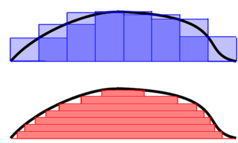
So for the Lebesgue integral, the range is partitioned into intervals, and so the region under the graph is partitioned into horizontal “slabs” (which may not be connected sets). The area of a small horizontal “slab” under the graph of $f$, of height $dy$, is equal to the measure of the slab’s width times $dy$:

\[\mu ( \{ x | f(x) > y \} ) dy.\]

The Lebesgue integral may then be defined by adding up the areas of these horizontal slabs. Lebesgue’s theory defines integrals for a class of functions called measurable functions: we start with a measure space $(E, X, μ)$ where $E$ is a set, $X$ is a $σ$-algebra of subsets of $E$, and $μ$ is a (non-negative) measure on $E$ defined on the sets of $X$². In the mathematical theory of probability, we confine our study to a probability measure μ, which satisfies $μ(E) = 1$, relations between measure theory and probability can be found in previous homeworks.

This kind of integral is important to us because it removes the dicotomy between discrete and continuous random variable, by generalizing the definitions based on a random variable distribution such as Expectation and Variance. For example, let $(E, S, μ)$ be a measure (probability) space, $X:E \to \Re$ a random variable. We define the expected value of $X$ as

\[EX = \int_E Xdμ\]

and

\[VX = \int_E (X - EX)^2 dμ\]

where E is a sample space, and it could be discrete or continuous.

Law of Large Numbers

It’s a theorem that describes the result of performing the same experiment a large number of times. According to the law, the average of the results obtained from a large number of trials should be close to the expected value and tends to become closer to the expected value as more trials are performed³. The LLN is important because it guarantees stable long-term results for the averages of some random events. For example, while a casino may lose money in a single spin of the roulette wheel, its earnings will tend towards a predictable percentage over a large number of spins. Importantly, the law applies only when a large number of observations are considered. There is no principle that a small number of observations will coincide with the expected value or that a streak of one value will immediately be “balanced” by the others.

There are two different versions of the law of large numbers that are described below. They are called the strong law of large numbers and the weak law of large numbers. Stated for the case where $X1, X2, \dots $ is an infinite sequence of independent and identically distributed (i.i.d.) Lebesgue integrable random variables with expected value $E(X_1) = E(X_2) = \dots = µ$, both versions of the law state that the sample average

\[{\bar X}_n={\frac {1}{n}}(X_1+ \dots + X_n)\]

converges to the expected value:

\(\bar X_n \to \mu \quad as \quad n \to \infty\).

(Lebesgue integrability of $X_i$ means that the expected value $E(X_i)$ exists according to Lebesgue integration and is finite). The difference between the strong and the weak version is concerned with the mode of convergence being asserted.

WLLN

The weak law of large numbers (also called Khinchin’s law) states that the sample average converges in probability towards the expected value \(\bar X_n \to \mu \quad as \quad n \to \infty\), that is, for any positive number $ε$, $\lim \limits_{n \to \infty} Pr(|{\bar X_n} - \mu| < ε) = 1$.

Interpreting this result, the weak law states that for any nonzero margin specified, no matter how small, with a sufficiently large sample there will be a very high probability that the average of the observations will be close to the expected value; that is, within the margin.

SLLN

The strong law of large numbers (also called Kolmogorov’s law) states that the sample average converges almost surely to the expected value: \(\bar X_n \to \mu \quad as \quad n \to \infty\). That is, $Pr(\lim \limits_{n \to \infty} {\bar X_n} = \mu) = 1$. What this means is that the probability that, as the number of trials n goes to infinity, the average of the observations converges to the expected value, is equal to one.

Chebyshev’s Inequality

If $X$ is any random variable with finite expected value $μ$ and finite non-zero variance $σ^2$, then for any $k>0$ we have \(P(|X - \mu| \ge kσ) \le \frac {1}{k^2}\)

Proof using Chebyshev’s Inequality

This proof uses the assumption of finite variance $Var(X_i) = σ^2$ (for all $i$). \(Var({\bar X_n}) = Var(\frac{1}{n}(X_1 + \dots + X_n)) = \frac{1}{n^2}Var(X_1 + \dots + X_n) = \frac{nσ^2}{n^2} = \frac{σ^2}{n}\)

The common mean μ of the sequence is the mean of the sample average: $E({\bar X_n}) = \mu$.

Using Chebyshev’s inequality on ${\bar X_n}$ results in

\(P(|{\bar X_n - \mu}| \ge ε) \le \frac{σ^2}{nε^2}\).

This may be used to obtain the following:

\(P(|{\bar X_n - \mu}| < ε) = 1 - P(|{\bar X_n - \mu}| \ge ε) \ge 1 - \frac{σ^2}{nε^2}\).

As n approaches infinity, the expression approaches 1. And by definition of convergence in probability, we have obtained \bar X_n \to \mu \quad when \quad n \to \infty.

Application

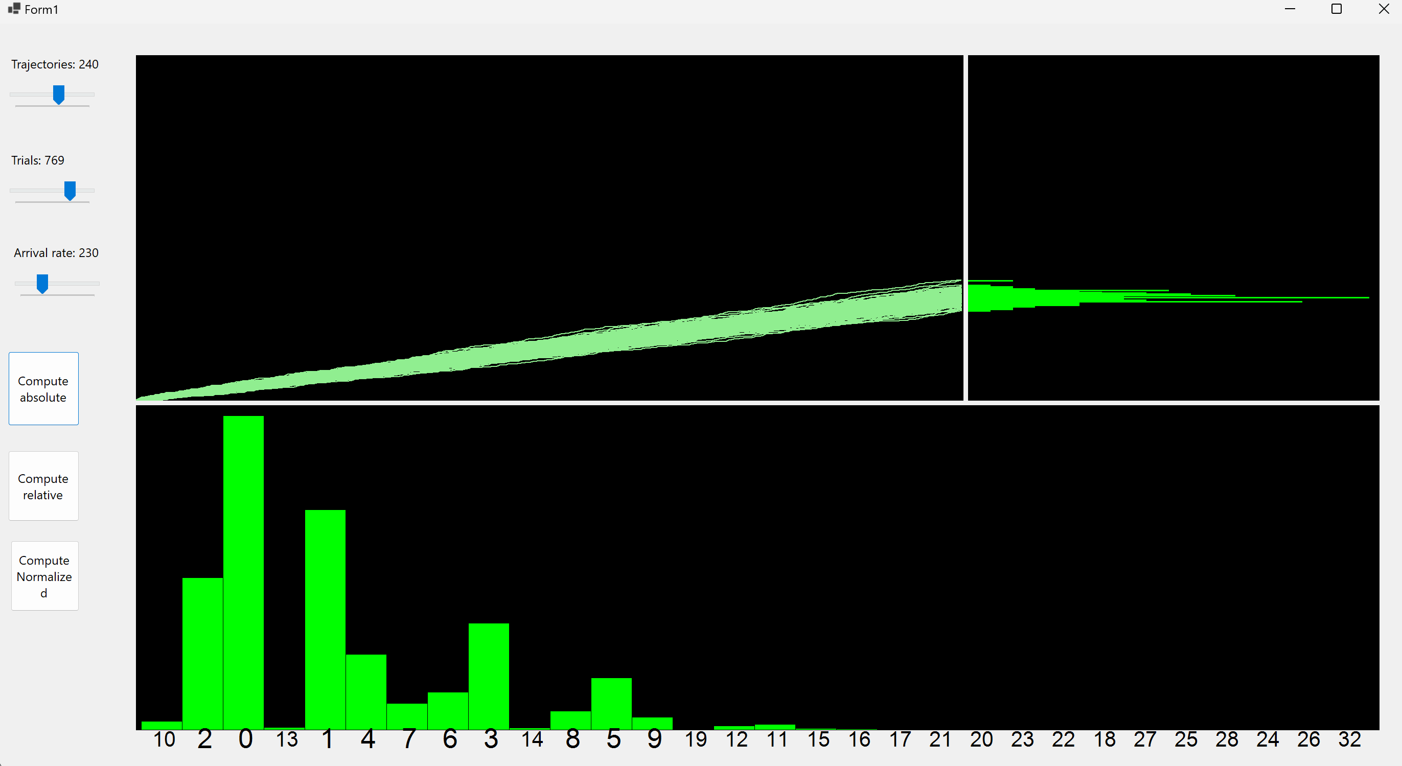
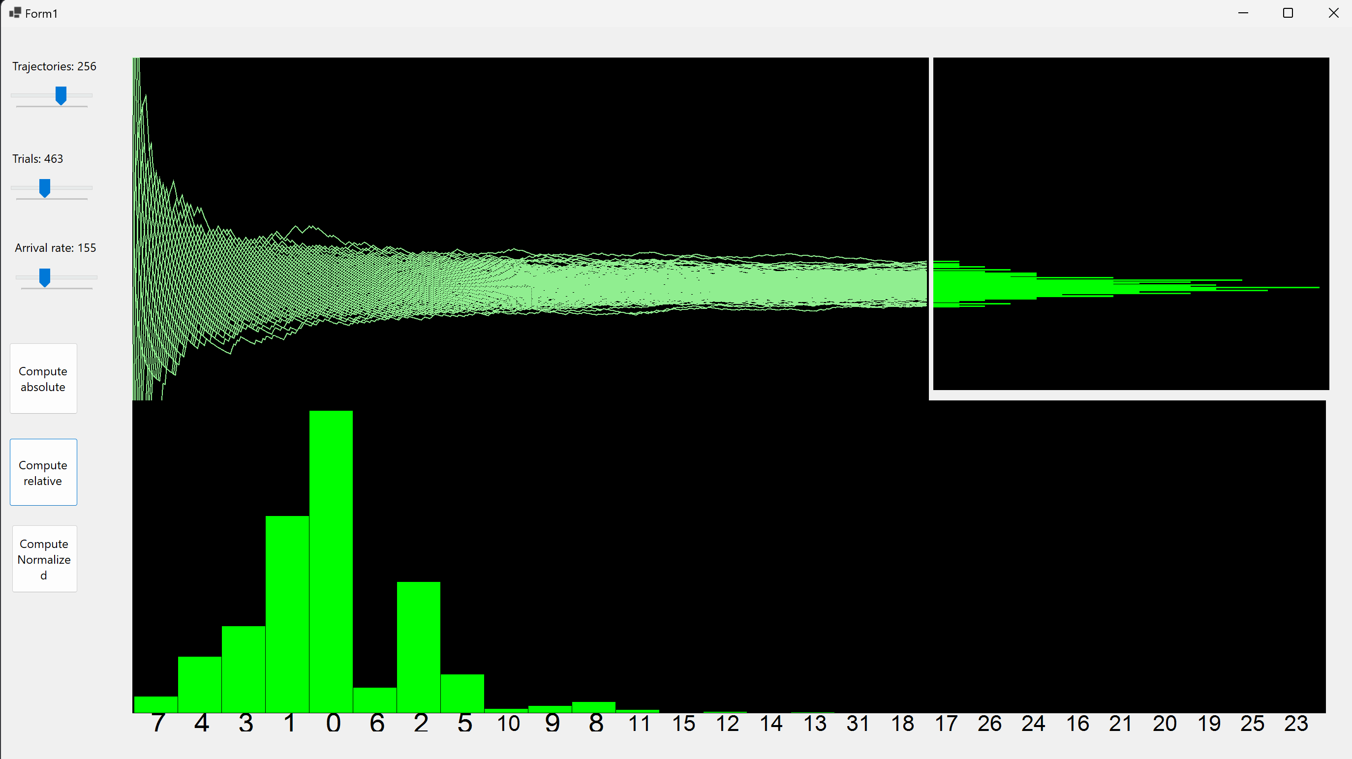
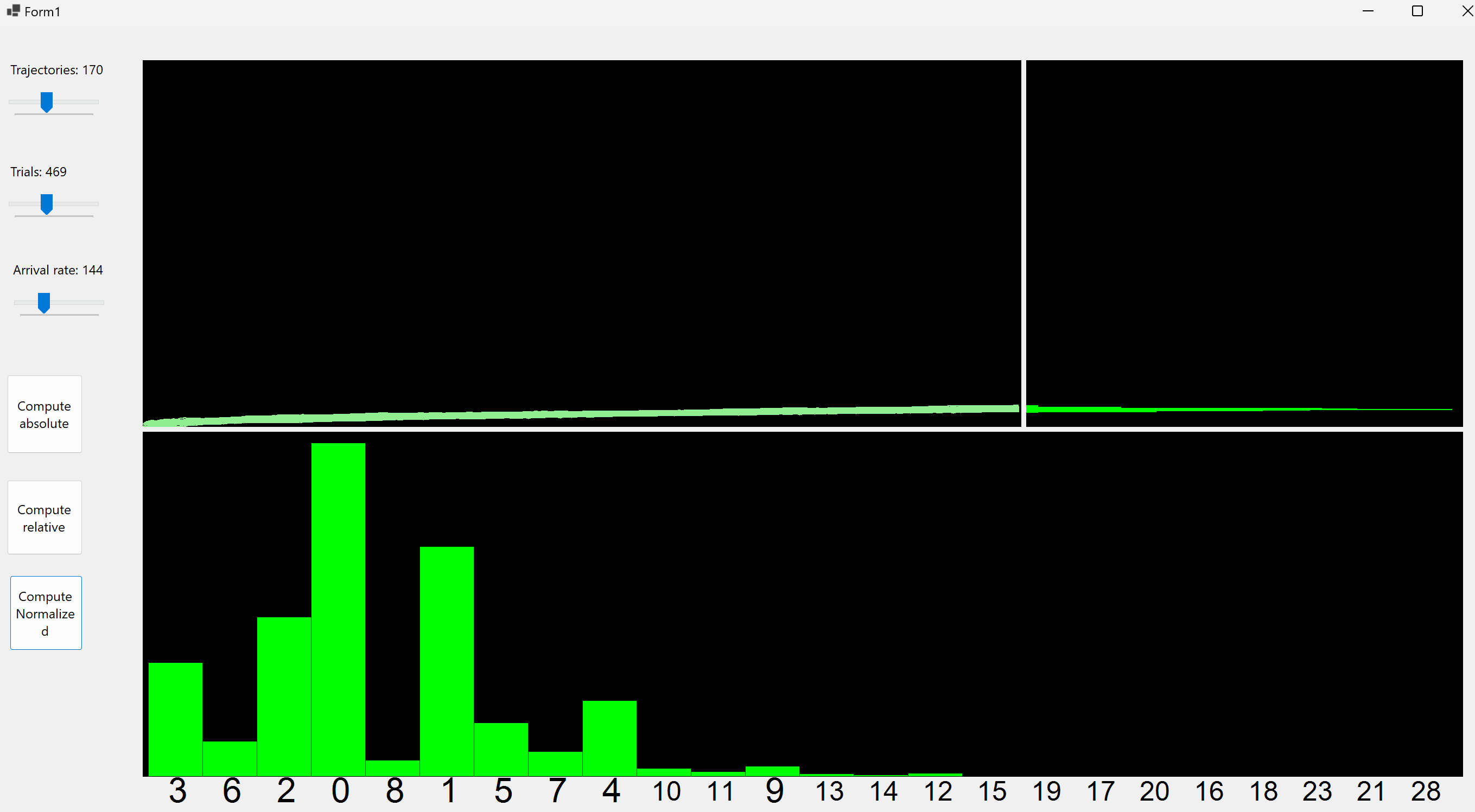
Following the homework 4 application, we compute the distribution of samples of coin tosses but this time with a success probability for each toss of λ/n. We also plot a p = SUM($X_i$) distribution, where $X_i$ are Bernoulli.

Code is avaible on github or can be downloaded with drive

---