HOMEWORK 08

Box-Muller Trasform and Marsaglia Polar Method

To change coordinates we used the following formulas (referring to the first application):

\[x = r \cos (\theta)\]

and

\[y = r \sin (\theta)\]

The polar coordinates are generated through a Random object, which return a double that falls inside $[0, 360°]$ for the angle and inside $[0, radius]$ for the module. We can notice that X and Y’s distributions have a so-called bell shape…they resemble two normal distributions! This is because we are simulating something that is very similar to a Box–Muller transform ¹: it is a random number sampling method for generating pairs of independent, standard, normally distributed random numbers, given a source of uniformly distributed random numbers. Suppose $U_1, U_2$ as independent samples chosen from the uniform distribution on the unit interval (0, 1):

\[Z_0 = R \cos (\Theta) = \sqrt {-2\ln U_1} {\cos 2\pi U_2}\]

and

\[Z_1 = R \sin (\Theta) = \sqrt {-2\ln U_1} {\sin 2\pi U_2}\]

Then $Z_0$ and $Z_1$ are independent random variables with a standard normal distribution. The difference we notice between our method and the Box-Muller method is that we obtain by the following formula: $R = rU_1$ instead of $R = \sqrt {-2\ln U_1}$

The polar form of this method is called the Marsaglia Polar Method²: again we use two uniform random variables $U_1$ and $U_2$ generate two normal random variables $X$ and $Y$. The polar method works by sampling random points (u, v) in the square −1 < x < 1, −1 < y < 1 until

\[0 < s = u^2 + v^2 < 1\]

We now identify the value of $s$ with that of $U_1$ and ${\theta\over 2\pi}$ with that of $U_2$ in the basic form. The values $\cos \theta = \cos{2\pi U_2}$ and $\sin \theta = \sin{2\pi U_2}$ in the basic form can be replaced with the ratios $\cos \theta = \frac{u}{R} = \frac{u}{\sqrt s}$ and $\sin \theta = \frac{v}{R} = \frac{v}{\sqrt s}$, respectively. The advantage is that calculating the trigonometric functions directly can be avoided. This is helpful when trigonometric functions are more expensive to compute than the single division that replaces each one.

Finally we obtain:

\[Z_0 = \sqrt {-2\ln U_1} {\cos 2\pi U_2} = \sqrt {-2\ln s}(\frac{u}{\sqrt s}) = u \sqrt{\frac{-2 \ln s}{s}}\]

and

\[Z_1 = \sqrt {-2\ln U_1} {\sin 2\pi U_2} = \sqrt {-2\ln s}(\frac{v}{\sqrt s}) = v \sqrt{\frac{-2 \ln s}{s}}\]

First App

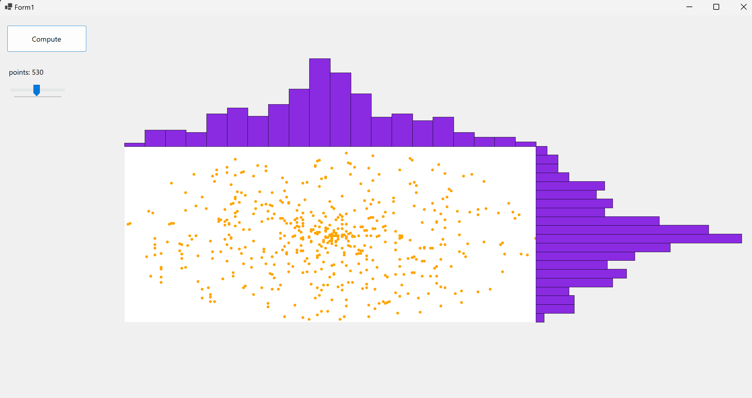
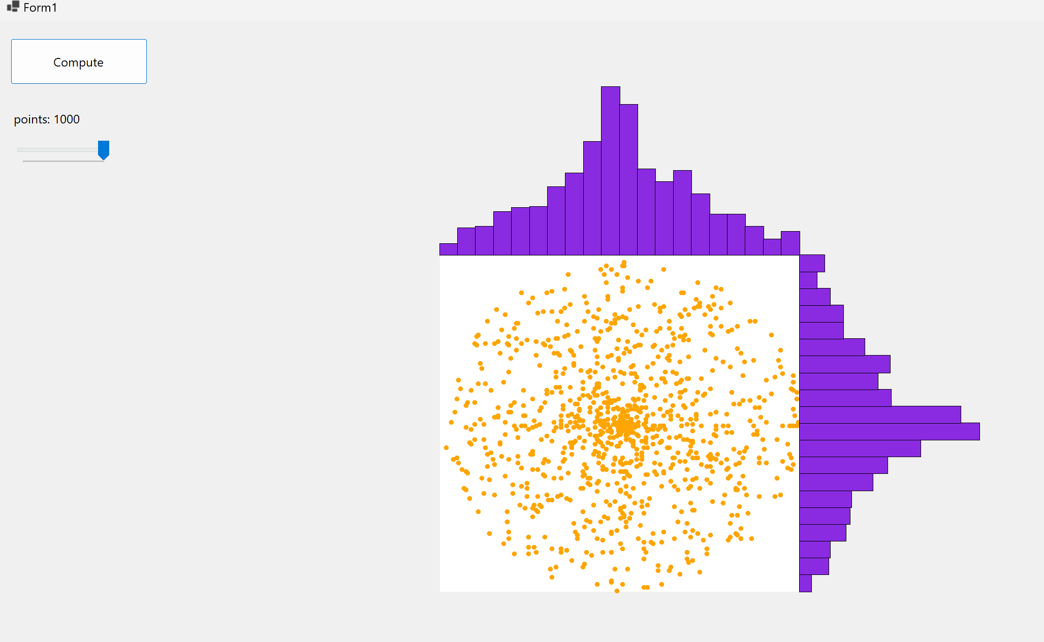
Here’s an application that generate random polar coordinates, transpose them into cartesians, plot them in a chart and plot X and Y variable’s distrubions on the side:

Code’s avaible on GitHub or Drive

Derivates of the Normal Distribution

In statistics, a normal distribution or Gaussian distribution is a type of continuous probability distribution for a real-valued random variable. The general form of its probability density function is:

\[f(x) = \frac{1}{\sigma\sqrt {2\pi}}e^{\frac{1}{2}(\frac{x - \mu}{\sigma})^2}\]

The parameter $\mu$ is the mean or expectation of the distribution, while the parameter \sigma is its standard deviation. The variance of the distribution is $\sigma ^{2}$. A random variable with a Gaussian distribution is said to be normally distributed, and is called a normal deviate.

Normal distributions are important in statistics and are often used in the natural and social sciences to represent real-valued random variables whose distributions are not known. Their importance is partly due to the central limit theorem³. It states that, under some conditions, the average of many samples (observations) of a random variable with finite mean and variance is itself a random variable—whose distribution converges to a normal distribution as the number of samples increases⁴. Therefore, physical quantities that are expected to be the sum of many independent processes, such as measurement errors, often have distributions that are nearly normal. We can say that most kinds of variables in natural and social sciences are normally or approximately normally distributed. Moreover, Gaussian distributions have some unique properties that are valuable in analytic studies. For instance, any linear combination of a fixed collection of normal deviates is a normal deviate.

Standard Normal Distribution

The simplest case of a normal distribution is known as the standard normal distribution or unit normal distribution. This is a special case when $\mu = 0$ and $\sigma =1$, and it is described by this probability density function (or density):

\[\phi(z) = \frac{e^{-z^2\over 2}}{\sqrt{2\pi}}\]

The variable $z$ has a mean of 0 and a variance and standard deviation of 1. The density $\phi (z)$ has its peak $1/{\sqrt {2\pi }}$ at $z=0$ and inflection points at $z = +1$ and $z = -1$.

Generalization and Notation

Every normal distribution is a version of the standard normal distribution, whose domain has been stretched by a factor $\sigma$ (the standard deviation) and then translated by $\mu$ (the mean value):

\[f(x | \mu, \sigma^2) = {1 \over\sigma}\phi(\frac{x - \mu}{\sigma})\]

The probability density must be scaled by $1/\sigma$ so that the integral is still 1. If $Z$ is a standard normal deviate, then $ X=\sigma Z+\mu$ will have a normal distribution with expected value $\mu$ and standard deviation $\sigma$. This is equivalent to saying that the “standard” normal distribution $Z$ can be scaled/stretched by a factor of $\sigma$ and shifted by $\mu$ to yield a different normal distribution, called $X$. Conversely, if $X$ is a normal deviate with parameters $\mu$ and $\sigma ^{2}$, then this $X$ distribution can be re-scaled and shifted via the formula $Z=\frac{(X-\mu )}{\sigma}$ to convert it to the “standard” normal distribution. This variate is also called the standardized form of $X$.

The normal distribution is often referred to as $N(\mu, \sigma^2)$. Thus when a random variable $X$ is normally distributed with mean $\mu$ and standard deviation $\sigma$, one may write $X \sim N(\mu, \sigma^2)$

De Moivre-Laplace Theorem

The de Moivre–Laplace theorem states that the normal distribution may be used as an approximation to the binomial distribution under certain conditions⁵. In particular, the theorem shows that the probability mass function of the random number of “successes” observed in a series of $n$ independent Bernoulli trials, each having probability $p$ of success (a binomial distribution with $n$ trials), converges to the probability density function of the normal distribution with mean $np$ and standard deviation ${\sqrt {np(1-p)}}$, as $n$ grows large, assuming $p$ is not 0 or 1.

This is one derivation of the particular Gaussian function used in the normal distribution.

As $n$ grows large, for $k$ in the neighborhood of $np$ we can approximate:

\[{n\choose k}p^{k}q^{n-k}\simeq{\frac{1}{\sqrt{2\pi npq}}}\,e^{-{\frac{(k-np)^{2}}{2npq}}},\qquad p+q=1,\ p,q>0\]

in the sense that the ratio of the left-hand side to the right-hand side converges to 1 as $n → ∞$

Gaussian Functions

In mathematics, a Gaussian function, often simply referred to as a Gaussian, is a function of the form

\[f(x) = ae^{-\frac{(x-b)^2}{2c^2}}\]

for arbitrary real constants a, b and non-zero c. Gaussian functions are often used to represent the probability density function of a normally distributed random variable with expected value $μ = b$ and variance $σ^2 = c^2$.

Second Application

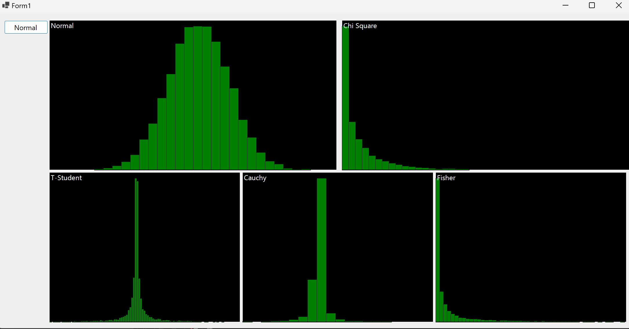
This application generates 10000 normal random variables, then computes Gaussian Distribution and the distributions of the following random variables: $X, X^2, X/Y^2, X^2/Y^2 , X/Y$

Avaible on GitHub or Drive

Find in the web what are the distributions that you just simulated

Chi-Square Distribution

Chi-square $(Χ^2)$ distributions are a family of continuous probability distributions, they’re widely used in hypothesis tests. Very few real-world observations follow a chi-square distribution. The main purpose of chi-square distributions is hypothesis testing, not describing real-world distributions⁶. Chi-square distributions are useful for hypothesis testing because of their close relationship to the standard normal distribution. The standard normal distribution, which is a normal distribution with a mean of zero and a variance of one, is central to many important statistical tests and theories. Imagine taking a random sample of a standard normal distribution $Z$. If you squared all the values in the sample, you would have the chi-square distribution with k = 1.

If $Z1, \ldots, Zk$ are independent, standard normal random variables, then the sum of their squares,

\[Q =\sum_{i=1}^{k}Z_{i}^{2}\]

is distributed according to the chi-squared distribution with $k$ degrees of freedom. This is usually denoted as

\[Q\sim\chi^{2}(k)\ \ {\text{or}}\ \ Q\sim\chi_{k}^{2}\]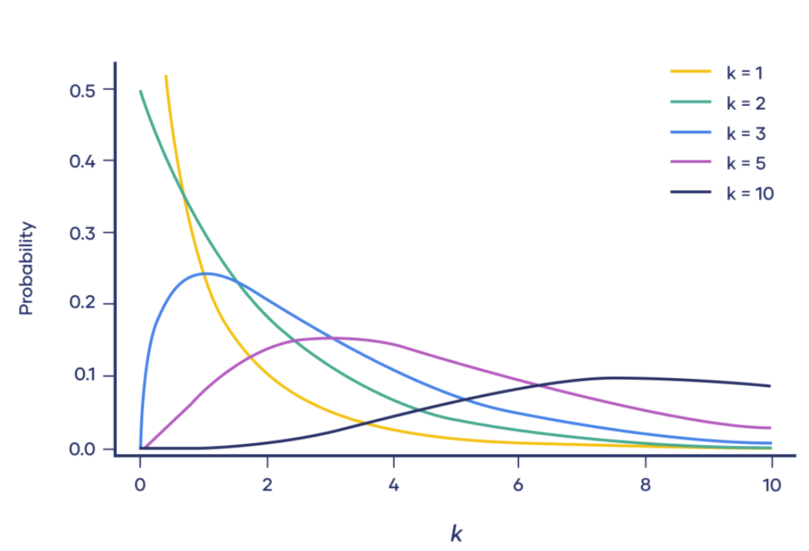

Cauchy Distribution

The Cauchy distribution is a family of continuous probably distributions which resemble the normal distribution family of curves. While the resemblance is there, it has a taller peak than a normal. And unlike the normal distribution, it’s fat tails decay much more slowly⁷. The Cauchy distribution $f(x;x_{0},\gamma )$ is the distribution of the x-intercept of a ray issuing from $(x_{0},\gamma )$ with a uniformly distributed angle. It is also the distribution of the ratio of two independent normally distributed random variables with mean zero.

The Cauchy distribution is often used in statistics as the canonical example of a “pathological” distribution since both its expected value and its variance are undefined.

The Cauchy distribution has the probability density function:

\[f(x;x_{0},\gamma)=\frac{1}{\pi\gamma\left[1+\left(\frac{x-x_{0}}{\gamma}\right)^{2}\right]}={1\over\pi\gamma}\left[{\gamma^{2}\over(x-x_{0})^{2}+\gamma^{2}}\right]\]

where $x_0$ is the location parameter, specifying the location of the peak of the distribution, and $\gamma$ is the scale parameter which specifies the half-width at half-maximum (HWHM), alternatively $2\gamma$ is full width at half maximum (FWHM). $\gamma$ is also equal to half the interquartile range and is sometimes called the probable error⁸.

T-Student Distribution

In probability and statistics, Student’s t-distribution (or simply the t-distribution) is any member of a family of continuous probability distributions that arise when estimating the mean of a normally distributed population in situations where the sample size is small and the population’s standard deviation is unknown⁹. If we take a sample of $n$ observations from a normal distribution, then the t-distribution with $\nu=n-1$ degrees of freedom can be defined as the distribution of the location of the sample mean relative to the true mean, divided by the sample standard deviation, after multiplying by the standardizing term ${\sqrt {n}}$. In this way, the t-distribution can be used to construct a confidence interval for the true mean.

The t-distribution is symmetric and bell-shaped, like the normal distribution. However, the t-distribution has heavier tails, meaning that it is more prone to producing values that fall far from its mean. This makes it useful for understanding the statistical behavior of certain types of ratios of random quantities, in which variation in the denominator is amplified and may produce outlying values when the denominator of the ratio falls close to zero. Let $ X_{1},\ldots ,X_{n}$ be independently and identically drawn from the distribution $X \sim N(\mu, \sigma^2)$, i.e. this is a sample of size $n$ from a normally distributed population with expected mean value $\mu$ and variance $\sigma ^{2}$ then the random variable

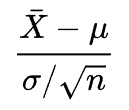
has a standard normal distribution (i.e. normal with expected mean 0 and variance 1) and

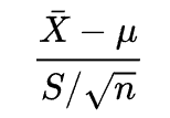
has a Student’s t-distribution with $n-1$ degrees of freedom, where $S$ is a (Bessel-corrected) sample variance.

Fisher-Snedecor Distribution

In probability theory, Fisher-Snedecor Distribution is a continuous distribution that regulates the ratio between two Chi-square random variables.

The F-distribution with d1 and d2 degrees of freedom is the distribution of

\[X={\frac {S_{1}/d_{1}}{S_{2}/d_{2}}}\]

where $S_{1}$ and $S_{2}$are independent random variables with chi-square distributions with respective degrees of freedom $ d_{1}$ and $d_{2}$¹⁰.

---